Introduction
My last articles looked at Real-Time Intelligence from a wide angle: how data flows from an API all the way to a data agent, and what the whole thing actually costs in Fabric. This time I’m zooming in on something smaller that you deal with every day: the KQL query itself.
There’s no shortage of tips on KQL performance. Put the time filter first, use has instead of contains, don’t join too early, do the expensive work at ingestion instead of in every query. Microsoft’s best practices say the same. But one thing was always missing for me: how much does it actually help? Are we talking a few percent, or is there a world of difference between a bad query and a good one?
That’s what I wanted to find out. So I built a test dataset with 100 million events, wrote a query that gets pretty much everything wrong, and improved it step by step. I measured every step: duration, CPU, memory, and how much data was read.
Why does this matter if an Eventhouse is billed by uptime and not per query? Because slow queries still cost you something: dashboards that refresh sluggishly, users who have to wait, and capacity that’s missing for other workloads. Especially when lots of people look at a Real-Time Dashboard at the same time, every bad query shows.
By the end of this article, you’ll know which optimizations make the biggest difference, in what order to tackle them, and how to measure your own queries. You’ll find the notebook and all the queries in my GitHub repo, so you can rebuild the test yourself.
The test setup
To show what an optimization does, you need a query that really hurts. My real project data didn’t work for that. The tables are too small, and the differences were just a few milliseconds. So I built my own dataset, big enough that bad KQL actually shows.
What you need
- A Fabric capacity. I ran the tests on an F64 (trial). The absolute times depend on the capacity size, so what matters most is how the steps compare to each other.
- A separate Eventhouse just for the test. Mine is called
eh_perf. All databases in an Eventhouse share the same compute. If I had loaded the test data into my existing Eventhouse, the test would have slowed down my other dashboards. - A Fabric notebook that generates the test data. You’ll find it in my GitHub repo.
- A KQL queryset to run the queries and measure them.
The data
The scenario is a web shop that tracks every click its customers make:
| Table | Rows | Content |
|---|---|---|
ShopEvents | 100 million | Page views, searches, cart, checkout, purchases, and errors over 90 days (Aug 18 to Nov 15, 2026) |
Users | 1 million | Customers with a segment (New, Regular, Loyal, VIP) |
Products | 1,000 | Products in 10 categories |
The events are spread out the way you’d expect in a real shop: 70% page views, 15% searches, 8% add to cart, 4% checkout, 2.5% purchases, and 0.5% errors.
I built a few typical traps into ShopEvents on purpose:
- The time is stored twice: as a proper
datetimecolumn and also as a Unix timestamp in milliseconds, the way it often comes from source systems. - Device, browser, and price are packed into a JSON column (
Payload). - There’s free text in
Messageand URLs, like you’d find in real logs.
How the data is generated
The notebook creates the data right inside the Eventhouse with KQL (range and .set-or-append), in ten chunks of 10 million rows each. Every chunk covers its own nine days. That part matters: the data ends up stored in time order, just like a real stream. Only then can Kusto skip entire blocks of data when you filter on time, and that’s one of the effects we want to measure.
On the F64, a chunk of 10 million rows is about 2.8 GB uncompressed and about 0.8 GB compressed, plus the index.
Before I had the notebook, I loaded the chunks by hand. I learned a few things along the way that went straight into the notebook:
- Only one load at a time. I wanted to start all ten chunks in parallel with
asyncto save time. But the Eventhouse only accepted one.set-or-appendand rejected all the others right away as “Throttled”. You still get an OperationId for every command, though. Whether it’s actually running, you only see in.show operations. That’s why the notebook loads the chunks strictly one after another and retries after a short wait if it gets throttled. - Data types have to match exactly. In KQL,
toint(rand(1000)) + 1returns along, because the1counts as along. The table expected anint, so the command failed with “Query schema does not match table schema”. The right way istoint(rand(1000) + 1). hasis notcontains. When I searched.show operationsfor my load commands, I got nothing back. I had filtered onhas "SetOrAppend", but the operation is calledTableSetOrAppend, andhasonly matches whole words. A nice preview of one of the things this article is about.- Use a fixed start date. My first commands calculated “today minus 90 days”. Since I didn’t load all the chunks on the same day, part of the data shifted by a day. So the notebook uses a fixed start date. It also checks before each chunk whether it’s already complete, so if something breaks, you just run it again.
How I measured
All queries answer the same question:
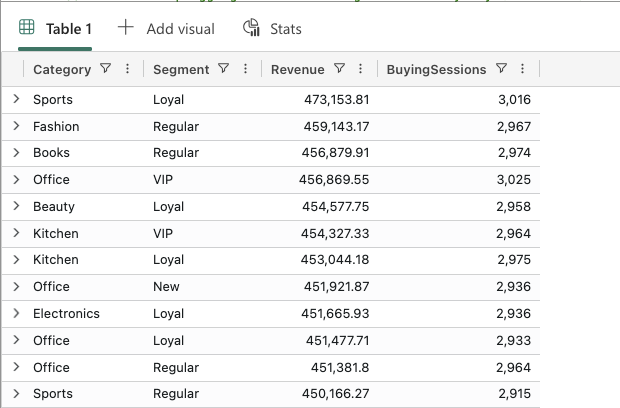
How much revenue and how many buying sessions did we have last week per product category and customer segment, counting only purchases on mobile devices?
“Last week” here means the last 7 days of the test data, starting Nov 9, 2026. I used a fixed date on purpose instead of ago(7d). Otherwise the result would depend on the day I run the query, and the runs wouldn’t be comparable.
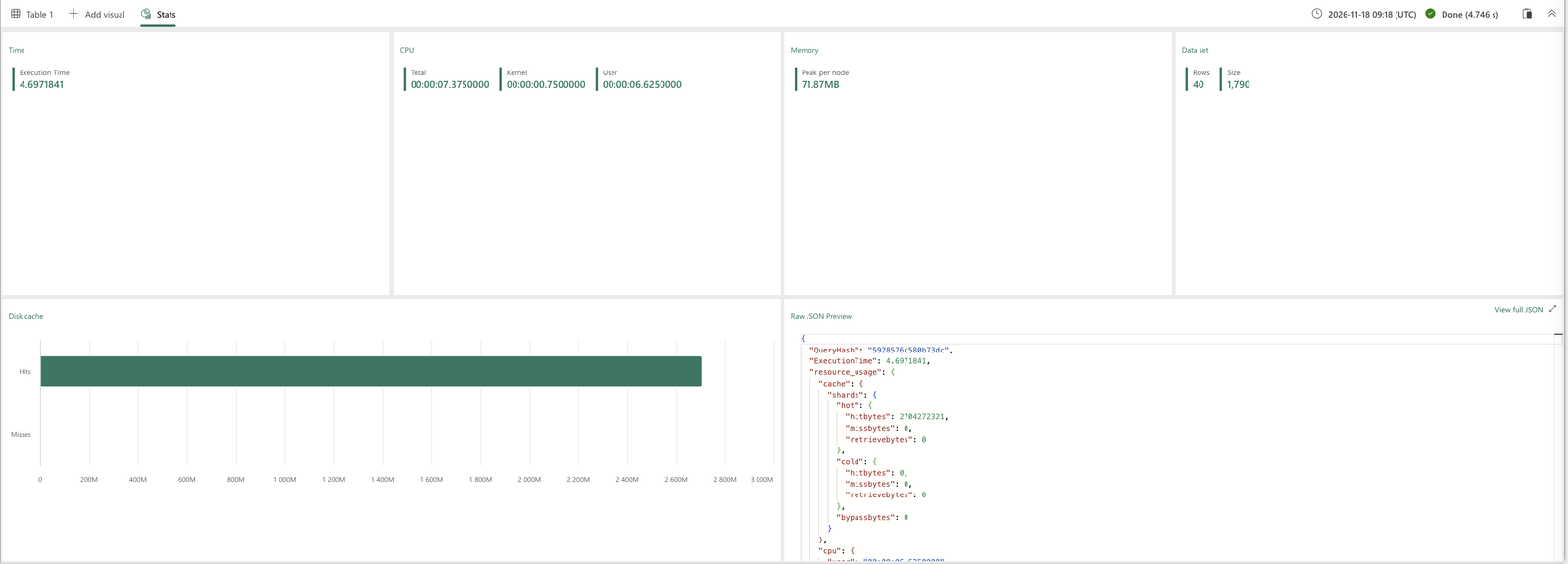
I ran every query at least three times and took the median, since the first run is often slower. The numbers come from the Stats tab in the queryset and from .show queries: duration, CPU time, memory, and how much data was read. To find the runs again later, every query starts with a tag like let _tag = "PERF-TEST Q0";.
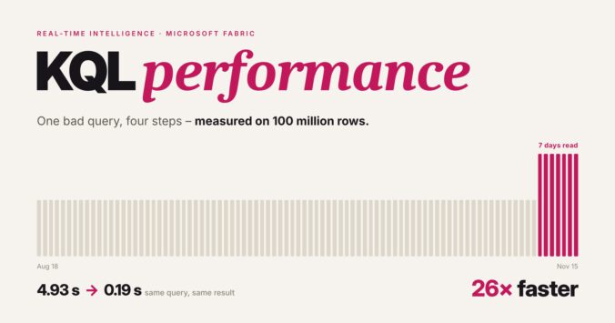
From 4.93 to 0.19 seconds, step by step
The starting point: everything you shouldn’t do
This is the kind of query that’s actually pretty common in real life. You start somewhere, pull in the columns you need one by one, join the master data, and filter at the end. It’s correct, it returns the right result. But it gets pretty much everything wrong that you can get wrong in KQL:
ShopEvents
| extend EventTime = unixtime_milliseconds_todatetime(EventTimeUnix)
| extend LocalTime = datetime_utc_to_local(EventTime, "Europe/Berlin")
| extend Device = tostring(Payload.device), Price = todouble(Payload.price)
| join kind=inner Users on UserId
| join kind=inner Products on ProductId
| where LocalTime >= datetime_utc_to_local(datetime(2026-11-09), "Europe/Berlin")
| where tolower(EventType) == "purchase" and Message contains "confirmed"
| where Device == "mobile"
| summarize Revenue = sum(Price) by Category, Segment, SessionId
| summarize Revenue = round(sum(Revenue), 2), BuyingSessions = count() by Category, Segment
| order by Revenue desc
What’s wrong here:
- The time filter comes at the very end, and it doesn’t run on the
datetimecolumn. It runs on a value that first has to be calculated from the Unix timestamp and converted to local time for every single row. - The JSON in
Payloadgets parsed for all 100 million rows, even though only about 116,000 are needed in the end. - The huge fact table sits on the left side of the join, and the join happens before anything is filtered.
tolower(...) ==andcontainsinstead of==andhas.- The aggregation runs in two steps over
SessionId, a column with a huge number of distinct values.
| Metric | Q0 |
|---|---|
| Duration | 4.93 s |
| CPU time | 7.42 s |
| Memory (peak per node) | 72 MB |
| Data read | 2.7 GB |
| Extents scanned | 11 of 11 |
| Rows scanned | 101 M of 101 M |
To be honest, I expected worse. Just under five seconds for 100 million rows isn’t a disaster. That’s partly because Kusto fixes some things on its own: it only reads the columns it actually needs, and the optimizer moves some filters forward by itself. Still, take a look at the last two rows of the table: the query reads every single row of all three tables. For a question that only cares about one week.
Step 1: Move the time filter to the top (Q1)
The first change is the smallest one, and it makes the biggest difference. Instead of filtering on a calculated local time at the very end, the filter now sits right after the table name, on the actual datetime column:
ShopEvents
| where Timestamp >= datetime(2026-11-09)
| extend Device = tostring(Payload.device), Price = todouble(Payload.price)
| join kind=inner Users on UserId
| join kind=inner Products on ProductId
| where tolower(EventType) == "purchase" and Message contains "confirmed"
| where Device == "mobile"
| summarize Revenue = sum(Price) by Category, Segment, SessionId
| summarize Revenue = round(sum(Revenue), 2), BuyingSessions = count() by Category, Segment
| order by Revenue desc
Why this helps so much: Kusto stores data in blocks called extents, and for every extent it knows the lowest and highest value of each datetime column. If the time filter runs on that column, Kusto doesn’t even have to open the extents outside the time range. With a calculated value like LocalTime, that doesn’t work. Every row has to be converted first before Kusto knows whether it’s needed at all.
| Metric | Q0 | Q1 |
|---|---|---|
| Duration | 4.93 s | 0.73 s |
| CPU time | 7.42 s | 0.83 s |
| Memory (peak per node) | 72 MB | 72 MB |
| Data read | 2.7 GB | 0.28 GB |
| Extents scanned | 11 of 11 | 3 of 11 |
| Rows scanned | 101 M | 11 M |
One line in a different place, and the query is 6.8 times faster. Kusto skips 8 of 11 extents. That’s also why I made sure the test data is stored in time order. With a real stream, you get that for free.
Step 2: Filter first, then join (Q2)
In the second step, all filters move in front of the joins, and I replaced the slow comparisons:
tolower(EventType) == "purchase"becomesEventType == "purchase"Message contains "confirmed"becomesMessage has "confirmed"
ShopEvents
| where Timestamp >= datetime(2026-11-09)
| where EventType == "purchase" and Message has "confirmed"
| extend Device = tostring(Payload.device)
| where Device == "mobile"
| extend Price = todouble(Payload.price)
| join kind=inner Users on UserId
| join kind=inner Products on ProductId
| summarize Revenue = sum(Price) by Category, Segment, SessionId
| summarize Revenue = round(sum(Revenue), 2), BuyingSessions = count() by Category, Segment
| order by Revenue desc
tolower() has to create a new string for every row. contains looks for any sequence of characters anywhere in the text. has, on the other hand, looks for whole words and can use the term index that Kusto builds for every string column. And because all filters now come first, the joins only have to work with the few rows that are actually left.
| Metric | Q1 | Q2 |
|---|---|---|
| Duration | 0.73 s | 0.55 s |
| CPU time | 0.83 s | 0.69 s |
| Memory (peak per node) | 72 MB | 72 MB |
| Data read | 0.28 GB | 0.19 GB |
| Extents scanned | 3 of 11 | 3 of 11 |
| Rows scanned | 11 M | 11 M |
About a quarter faster again, and now 9 times faster than where we started. The number of extents stays the same, since the time filter still decides that. But inside those extents, Kusto touches a lot less data.
Step 3: Tuning the joins, with a surprise (Q3)
Microsoft’s best practices say this about joins:
- use
lookupinstead ofjoinwhen the right table is small, - and use
hint.strategy=broadcastwhen the left side is small.
On top of that, I added a project to keep only the columns I need, and a single aggregation with count_distinct() instead of the two steps over SessionId.
ShopEvents
| where Timestamp >= datetime(2026-11-09)
| where EventType == "purchase" and Message has "confirmed"
| where Payload has "mobile"
| where tostring(Payload.device) == "mobile"
| project SessionId, UserId, ProductId, Price = todouble(Payload.price)
| lookup kind=inner (Products | project ProductId, Category) on ProductId
| join kind=inner hint.strategy=broadcast (Users | project UserId, Segment) on UserId
| summarize Revenue = round(sum(Price), 2), BuyingSessions = count_distinct(SessionId) by Category, Segment
| order by Revenue desc
One more small trick in there: where Payload has "mobile" runs before the JSON gets parsed. It’s a cheap text check that throws out most rows early, so tostring(Payload.device) only has to run on the rest.
| Metric | Q2 | Q3 (broadcast) | Q3b (no hint) |
|---|---|---|---|
| Duration | 0.55 s | 0.67 s | 0.56 s |
| CPU time | 0.69 s | 0.61 s | 0.63 s |
| Memory (peak per node) | 72 MB | 39 MB | 88 MB |
| Network between nodes | 2 KB | 5 MB | 22 KB |
Q3 is slower than Q2. The last row shows why: with a broadcast join, Kusto sends the left side – the filtered purchases – to all nodes. That’s about 5 MB here, and sending it costs more time than the join saves. In return, memory use drops by almost half.
To be sure, I ran the same query without the broadcast hint (Q3b). It’s as fast as Q2, but it uses more memory than any other query in the test.
For me, this is the most interesting finding of the whole test: join hints aren’t a turbo button, they’re a trade-off. With this amount of data, they don’t make anything faster. They pay off when memory gets tight, for example when lots of queries run at the same time on a small capacity. There’s no way around it: measure instead of guessing.
Step 4: Do the expensive work once, at ingestion (Q4)
Up to this point, every query still reads the raw data. It picks the purchases out of all events and parses the JSON in Payload for every row. And it does that every single time it runs, including every time a dashboard refreshes.
With an update policy, that happens only once, when the data is loaded. New events land in ShopEvents, and Kusto automatically writes the purchases, with the columns already extracted, into a separate Purchases table:
.create table Purchases (Timestamp: datetime, SessionId: string, UserId: string, ProductId: int,
                         Device: string, Price: real)

.create-or-alter function with (folder = "UpdatePolicies") ExtractPurchases() {
    ShopEvents
    | where EventType == "purchase"
    | project Timestamp, SessionId, UserId, ProductId,
              Device = tostring(Payload.device), Price = todouble(Payload.price)
}

.alter table Purchases policy update
@'[{"IsEnabled": true, "Source": "ShopEvents", "Query": "ExtractPurchases()", "IsTransactional": false}]'
An update policy only works on data that arrives after it’s created. For the data that was already there, I filled the table once:
.set-or-append Purchases <| ExtractPurchases()That gave me 2,501,223 purchases, almost exactly the 2.5% from the test data. The query itself becomes short and simple:
Purchases
| where Timestamp >= datetime(2026-11-09)
| where Device == "mobile"
| lookup kind=inner (Products | project ProductId, Category) on ProductId
| join kind=inner hint.strategy=broadcast (Users | project UserId, Segment) on UserId
| summarize Revenue = round(sum(Price), 2), BuyingSessions = count_distinct(SessionId) by Category, Segment
| order by Revenue desc| Metric | Q0 | Q4 |
|---|---|---|
| Duration | 4.93 s | 0.19 s |
| CPU time | 7.42 s | 0.09 s |
| Memory (peak per node) | 72 MB | 29 MB |
| Data read | 2.7 GB | 0.016 GB |
| Rows scanned | 101 M | 3.1 M |
26 times faster than the starting point, with about 80 times less CPU and more than 170 times less data read. The price: a bit of extra storage for the Purchases table and a little compute time during ingestion. For a query that a dashboard runs every few seconds, that pays off right away.
The results at a glance
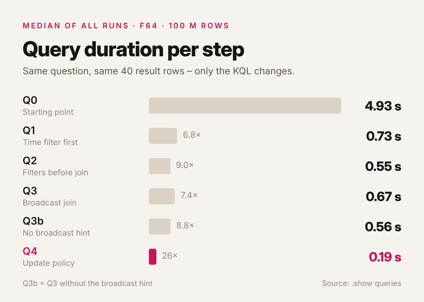
| Step | Duration | CPU time | Memory | Factor |
|---|---|---|---|---|
| Q0 – starting point | 4.93 s | 7.42 s | 72 MB | 1× |
| Q1 – time filter first | 0.73 s | 0.83 s | 72 MB | 6.8× |
| Q2 – filters before the join | 0.55 s | 0.69 s | 72 MB | 9.0× |
| Q3 – lookup + broadcast join | 0.67 s | 0.61 s | 39 MB | 7.4× |
| Q3b – lookup, no hint | 0.56 s | 0.63 s | 88 MB | 8.8× |
| Q4 – update policy | 0.19 s | 0.09 s | 29 MB | 26× |
Two steps make the real difference: putting the time filter first (almost 7 times faster) and moving the expensive work into ingestion with an update policy (almost 3 times on top). Everything in between helps a little, or, in the case of the join hint, is a trade-off rather than a win.
What I learned
- A time filter on the
datetimecolumn is the biggest single lever. One line in the right place makes the query almost 7 times faster. It also matters that the data is stored in time order, which a real stream gives you for free. - Expensive work belongs in ingestion, not in every query. Parsing JSON, converting times, pre-filtering data: with an update policy, that happens once instead of on every run.
- Not every best practice makes things faster. The broadcast join saved memory here and cost time. Join hints are a trade-off you have to measure for your own data.
dcount()is fast, but it’s an estimate. My first version of Q3 and Q4 useddcount(). When I compared the results with the starting point, 37 of 40 rows had slightly different session counts. If the numbers have to match exactly, usecount_distinct(). In this test, it cost practically no extra time.- Kusto is more forgiving than you’d think. Even the bad query ran in under 5 seconds, because Kusto only reads the columns it needs and fixes some mistakes on its own. But that’s no reason to rely on it. Once lots of users hit the same dashboard, every second counts.
- Measuring is easier than you’d expect. The Stats tab in the queryset and
.show queriesgive you everything you need. With a tag in the query text, you find your own runs right away.
Conclusion
Most of the speed in this test didn’t come from clever tricks. It came from two simple rules: filter on time first, and don’t make every query do work that could have been done once at ingestion. Together, that took the same query from almost 5 seconds down to 0.19 seconds.
The broadcast join was a good reminder that best practices are a starting point, not a guarantee. What helps depends on your data, your capacity and how many people run the query at the same time. So the most useful habit I took away from this is a simple one: look at the Stats tab before and after every change.
Further reading
Microsoft documentation
- Best practices for KQL queries – the official list this test is based on
- Extents overview – how Kusto stores data and why time filters can skip it
- String operators – why
hasis faster thancontains - lookup operator – joining small dimension tables
- Broadcast join – when the broadcast hint helps and when it doesn’t
- Update policy overview – transforming data at ingestion
- .show queries command – finding and measuring your own queries
More on Real-Time Intelligence on this blog
Try it yourself
Everything you need to rebuild the test is in my GitHub repo: ms-fabric / real-time-intelligence-kql-performance
generate_perf_demo_data.ipynbis a Fabric notebook that generates the 100 million test events, the users and the products in your own Eventhouse. It loads the data in chunks, one after another, and you can simply run it again if it gets interrupted.kql_performance_queries.kqlhas all queries from Q0 to Q4 (plus Q3b without the broadcast hint), the update policy and the measurement query with.show queries.
Use a separate Eventhouse for the test so it doesn’t slow down your other workloads. Run the notebook, run the queries, and compare your numbers with mine. When you’re done, drop the tables. I’d be curious how the numbers look on a smaller capacity like an F2 or F8.